14. Optimal Investment#
GPU
This lecture was built using a machine with JAX installed and access to a GPU.
To run this lecture on Google Colab, click on the “play” icon top right, select Colab, and set the runtime environment to include a GPU.
To run this lecture on your own machine, you need to install Google JAX.
In addition to JAX and Anaconda, this lecture will need the following libraries:
!pip install --upgrade quantecon
Show code cell output
Requirement already satisfied: quantecon in /home/runner/miniconda3/envs/quantecon/lib/python3.13/site-packages (0.10.1)
Requirement already satisfied: numba>=0.49.0 in /home/runner/miniconda3/envs/quantecon/lib/python3.13/site-packages (from quantecon) (0.61.0)
Requirement already satisfied: numpy>=1.17.0 in /home/runner/miniconda3/envs/quantecon/lib/python3.13/site-packages (from quantecon) (2.1.3)
Requirement already satisfied: requests in /home/runner/miniconda3/envs/quantecon/lib/python3.13/site-packages (from quantecon) (2.32.3)
Requirement already satisfied: scipy>=1.5.0 in /home/runner/miniconda3/envs/quantecon/lib/python3.13/site-packages (from quantecon) (1.15.3)
Requirement already satisfied: sympy in /home/runner/miniconda3/envs/quantecon/lib/python3.13/site-packages (from quantecon) (1.13.3)
Requirement already satisfied: llvmlite<0.45,>=0.44.0dev0 in /home/runner/miniconda3/envs/quantecon/lib/python3.13/site-packages (from numba>=0.49.0->quantecon) (0.44.0)
Requirement already satisfied: charset-normalizer<4,>=2 in /home/runner/miniconda3/envs/quantecon/lib/python3.13/site-packages (from requests->quantecon) (3.3.2)
Requirement already satisfied: idna<4,>=2.5 in /home/runner/miniconda3/envs/quantecon/lib/python3.13/site-packages (from requests->quantecon) (3.7)
Requirement already satisfied: urllib3<3,>=1.21.1 in /home/runner/miniconda3/envs/quantecon/lib/python3.13/site-packages (from requests->quantecon) (2.3.0)
Requirement already satisfied: certifi>=2017.4.17 in /home/runner/miniconda3/envs/quantecon/lib/python3.13/site-packages (from requests->quantecon) (2025.4.26)
Requirement already satisfied: mpmath<1.4,>=1.1.0 in /home/runner/miniconda3/envs/quantecon/lib/python3.13/site-packages (from sympy->quantecon) (1.3.0)
We study a monopolist who faces inverse demand curve
where
We assume that
Current profits are
Combining with the demand curve and writing
The firm maximizes present value of expected discounted profits. The Bellman equation is
We discretize y_grid.
In essence, the firm tries to choose output close to the monopolist profit maximizer, given
Let’s begin with the following imports
import quantecon as qe
import jax
import jax.numpy as jnp
import matplotlib.pyplot as plt
from time import time
Let’s check the GPU we are running
!nvidia-smi
Mon Oct 27 03:48:54 2025
+-----------------------------------------------------------------------------------------+
| NVIDIA-SMI 575.51.03              Driver Version: 575.51.03      CUDA Version: 12.9     |
|-----------------------------------------+------------------------+----------------------+
| GPU  Name                 Persistence-M | Bus-Id          Disp.A | Volatile Uncorr. ECC |
| Fan  Temp   Perf          Pwr:Usage/Cap |           Memory-Usage | GPU-Util  Compute M. |
|                                         |                        |               MIG M. |
|=========================================+========================+======================|
|   0  Tesla T4                       Off |   00000000:00:1E.0 Off |                    0 |
| N/A   33C    P8             15W /   70W |       0MiB /  15360MiB |      0%      Default |
|                                         |                        |                  N/A |
+-----------------------------------------+------------------------+----------------------+

+-----------------------------------------------------------------------------------------+
| Processes:                                                                              |
|  GPU   GI   CI              PID   Type   Process name                        GPU Memory |
|        ID   ID                                                               Usage      |
|=========================================================================================|
|  No running processes found                                                             |
+-----------------------------------------------------------------------------------------+
We will use 64 bit floats with JAX in order to increase the precision.
jax.config.update("jax_enable_x64", True)
Let’s define a function to create an investment model using the given parameters.
def create_investment_model(
        r=0.01,                              # Interest rate
        a_0=10.0, a_1=1.0,                   # Demand parameters
        γ=25.0, c=1.0,                       # Adjustment and unit cost
        y_min=0.0, y_max=20.0, y_size=100,   # Grid for output
        ρ=0.9, ν=1.0,                        # AR(1) parameters
        z_size=150):                         # Grid size for shock
    """
    A function that takes in parameters and returns an instance of Model that
    contains data for the investment problem.
    """
    β = 1 / (1 + r)
    y_grid = jnp.linspace(y_min, y_max, y_size)
    mc = qe.tauchen(z_size, ρ, ν)
    z_grid, Q = mc.state_values, mc.P

    # Break up parameters into static and nonstatic components
    constants = β, a_0, a_1, γ, c
    sizes = y_size, z_size
    arrays = y_grid, z_grid, Q

    # Shift arrays to the device (e.g., GPU)
    arrays = tuple(map(jax.device_put, arrays))
    return constants, sizes, arrays
Let’s re-write the vectorized version of the right-hand side of the Bellman equation (before maximization), which is a 3D array representing
for all
def B(v, constants, sizes, arrays):
    """
    A vectorized version of the right-hand side of the Bellman equation
    (before maximization)
    """

    # Unpack
    β, a_0, a_1, γ, c = constants
    y_size, z_size = sizes
    y_grid, z_grid, Q = arrays

    # Compute current rewards r(y, z, yp) as array r[i, j, ip]
    y  = jnp.reshape(y_grid, (y_size, 1, 1))    # y[i]   ->  y[i, j, ip]
    z  = jnp.reshape(z_grid, (1, z_size, 1))    # z[j]   ->  z[i, j, ip]
    yp = jnp.reshape(y_grid, (1, 1, y_size))    # yp[ip] -> yp[i, j, ip]
    r = (a_0 - a_1 * y + z - c) * y - γ * (yp - y)**2

    # Calculate continuation rewards at all combinations of (y, z, yp)
    v = jnp.reshape(v, (1, 1, y_size, z_size))  # v[ip, jp] -> v[i, j, ip, jp]
    Q = jnp.reshape(Q, (1, z_size, 1, z_size))  # Q[j, jp]  -> Q[i, j, ip, jp]
    EV = jnp.sum(v * Q, axis=3)                 # sum over last index jp

    # Compute the right-hand side of the Bellman equation
    return r + β * EV

# Create a jitted function
B = jax.jit(B, static_argnums=(2,))
We define a function to compute the current rewards
def compute_r_σ(σ, constants, sizes, arrays):
    """
    Compute the array r_σ[i, j] = r[i, j, σ[i, j]], which gives current
    rewards given policy σ.
    """

    # Unpack model
    β, a_0, a_1, γ, c = constants
    y_size, z_size = sizes
    y_grid, z_grid, Q = arrays

    # Compute r_σ[i, j]
    y = jnp.reshape(y_grid, (y_size, 1))
    z = jnp.reshape(z_grid, (1, z_size))
    yp = y_grid[σ]
    r_σ = (a_0 - a_1 * y + z - c) * y - γ * (yp - y)**2

    return r_σ


# Create the jitted function
compute_r_σ = jax.jit(compute_r_σ, static_argnums=(2,))
Define the Bellman operator.
def T(v, constants, sizes, arrays):
    """The Bellman operator."""
    return jnp.max(B(v, constants, sizes, arrays), axis=2)

T = jax.jit(T, static_argnums=(2,))
The following function computes a v-greedy policy.
def get_greedy(v, constants, sizes, arrays):
    "Computes a v-greedy policy, returned as a set of indices."
    return jnp.argmax(B(v, constants, sizes, arrays), axis=2)

get_greedy = jax.jit(get_greedy, static_argnums=(2,))
Define the
def T_σ(v, σ, constants, sizes, arrays):
    """The σ-policy operator."""

    # Unpack model
    β, a_0, a_1, γ, c = constants
    y_size, z_size = sizes
    y_grid, z_grid, Q = arrays

    r_σ = compute_r_σ(σ, constants, sizes, arrays)

    # Compute the array v[σ[i, j], jp]
    zp_idx = jnp.arange(z_size)
    zp_idx = jnp.reshape(zp_idx, (1, 1, z_size))
    σ = jnp.reshape(σ, (y_size, z_size, 1))
    V = v[σ, zp_idx]

    # Convert Q[j, jp] to Q[i, j, jp]
    Q = jnp.reshape(Q, (1, z_size, z_size))

    # Calculate the expected sum Σ_jp v[σ[i, j], jp] * Q[i, j, jp]
    Ev = jnp.sum(V * Q, axis=2)

    return r_σ + β * Ev

T_σ = jax.jit(T_σ, static_argnums=(3,))
Next, we want to computes the lifetime value of following policy
This lifetime value is a function
We wish to solve this equation for
Suppose we define the linear operator
With this notation, the problem is to solve for
In vector for this is
JAX allows us to solve linear systems defined in terms of operators; the first
step is to define the function
def L_σ(v, σ, constants, sizes, arrays):

    β, a_0, a_1, γ, c = constants
    y_size, z_size = sizes
    y_grid, z_grid, Q = arrays

    # Set up the array v[σ[i, j], jp]
    zp_idx = jnp.arange(z_size)
    zp_idx = jnp.reshape(zp_idx, (1, 1, z_size))
    σ = jnp.reshape(σ, (y_size, z_size, 1))
    V = v[σ, zp_idx]

    # Expand Q[j, jp] to Q[i, j, jp]
    Q = jnp.reshape(Q, (1, z_size, z_size))

    # Compute and return v[i, j] - β Σ_jp v[σ[i, j], jp] * Q[j, jp]
    return v - β * jnp.sum(V * Q, axis=2)

L_σ = jax.jit(L_σ, static_argnums=(3,))
Now we can define a function to compute
def get_value(σ, constants, sizes, arrays):

    # Unpack
    β, a_0, a_1, γ, c = constants
    y_size, z_size = sizes
    y_grid, z_grid, Q = arrays

    r_σ = compute_r_σ(σ, constants, sizes, arrays)

    # Reduce L_σ to a function in v
    partial_L_σ = lambda v: L_σ(v, σ, constants, sizes, arrays)

    return jax.scipy.sparse.linalg.bicgstab(partial_L_σ, r_σ)[0]

get_value = jax.jit(get_value, static_argnums=(2,))
We use successive approximation for VFI.
def successive_approx_jax(T,                     # Operator (callable)
                          x_0,                   # Initial condition
                          tol=1e-6,              # Error tolerance
                          max_iter=10_000):      # Max iteration bound
    def body_fun(k_x_err):
        k, x, error = k_x_err
        x_new = T(x)
        error = jnp.max(jnp.abs(x_new - x))
        return k + 1, x_new, error

    def cond_fun(k_x_err):
        k, x, error = k_x_err
        return jnp.logical_and(error > tol, k < max_iter)

    k, x, error = jax.lax.while_loop(cond_fun, body_fun, (1, x_0, tol + 1))
    return x

successive_approx_jax = jax.jit(successive_approx_jax, static_argnums=(0,))
For OPI we’ll add a compiled routine that computes
def iterate_policy_operator(σ, v, m, params, sizes, arrays):

    def update(i, v):
        v = T_σ(v, σ, params, sizes, arrays)
        return v

    v = jax.lax.fori_loop(0, m, update, v)
    return v

iterate_policy_operator = jax.jit(iterate_policy_operator,
                                  static_argnums=(4,))
Finally, we introduce the solvers that implement VFI, HPI and OPI.
def value_function_iteration(model, tol=1e-5):
    """
    Implements value function iteration.
    """
    params, sizes, arrays = model
    vz = jnp.zeros(sizes)
    _T = lambda v: T(v, params, sizes, arrays)
    v_star = successive_approx_jax(_T, vz, tol=tol)
    return get_greedy(v_star, params, sizes, arrays)
For OPI we will use a compiled JAX lax.while_loop operation to speed execution.
def opi_loop(params, sizes, arrays, m, tol, max_iter):
    """
    Implements optimistic policy iteration (see dp.quantecon.org) with
    step size m.

    """
    v_init = jnp.zeros(sizes)

    def condition_function(inputs):
        i, v, error = inputs
        return jnp.logical_and(error > tol, i < max_iter)

    def update(inputs):
        i, v, error = inputs
        last_v = v
        σ = get_greedy(v, params, sizes, arrays)
        v = iterate_policy_operator(σ, v, m, params, sizes, arrays)
        error = jnp.max(jnp.abs(v - last_v))
        i += 1
        return i, v, error

    num_iter, v, error = jax.lax.while_loop(condition_function,
                                            update,
                                            (0, v_init, tol + 1))

    return get_greedy(v, params, sizes, arrays)

opi_loop = jax.jit(opi_loop, static_argnums=(1,))
Here’s a friendly interface to OPI
def optimistic_policy_iteration(model, m=10, tol=1e-5, max_iter=10_000):
    params, sizes, arrays = model
    σ_star = opi_loop(params, sizes, arrays, m, tol, max_iter)
    return σ_star
Here’s HPI
def howard_policy_iteration(model, maxiter=250):
    """
    Implements Howard policy iteration (see dp.quantecon.org)
    """
    params, sizes, arrays = model
    σ = jnp.zeros(sizes, dtype=int)
    i, error = 0, 1.0
    while error > 0 and i < maxiter:
        v_σ = get_value(σ, params, sizes, arrays)
        σ_new = get_greedy(v_σ, params, sizes, arrays)
        error = jnp.max(jnp.abs(σ_new - σ))
        σ = σ_new
        i = i + 1
        print(f"Concluded loop {i} with error {error}.")
    return σ
model = create_investment_model()
constants, sizes, arrays = model
β, a_0, a_1, γ, c = constants
y_size, z_size = sizes
y_grid, z_grid, Q = arrays
print("Starting HPI.")
%time σ_star_hpi = howard_policy_iteration(model).block_until_ready()
Show code cell output
Starting HPI.
Concluded loop 1 with error 50.
Concluded loop 2 with error 26.
Concluded loop 3 with error 17.
Concluded loop 4 with error 10.
Concluded loop 5 with error 7.
Concluded loop 6 with error 4.
Concluded loop 7 with error 3.
Concluded loop 8 with error 1.
Concluded loop 9 with error 1.
Concluded loop 10 with error 1.
Concluded loop 11 with error 1.
Concluded loop 12 with error 0.
CPU times: user 793 ms, sys: 103 ms, total: 897 ms
Wall time: 1.03 s
# Now time it without compile time
start = time()
σ_star_hpi = howard_policy_iteration(model).block_until_ready()
hpi_without_compile = time() - start
print(σ_star_hpi)
print(f"HPI completed in {hpi_without_compile} seconds.")
Concluded loop 1 with error 50.
Concluded loop 2 with error 26.
Concluded loop 3 with error 17.
Concluded loop 4 with error 10.
Concluded loop 5 with error 7.
Concluded loop 6 with error 4.
Concluded loop 7 with error 3.
Concluded loop 8 with error 1.
Concluded loop 9 with error 1.
Concluded loop 10 with error 1.
Concluded loop 11 with error 1.
Concluded loop 12 with error 0.
[[ 2  2  2 ...  6  6  6]
 [ 3  3  3 ...  7  7  7]
 [ 4  4  4 ...  7  7  7]
 ...
 [82 82 82 ... 86 86 86]
 [83 83 83 ... 86 86 86]
 [84 84 84 ... 87 87 87]]
HPI completed in 0.14738965034484863 seconds.
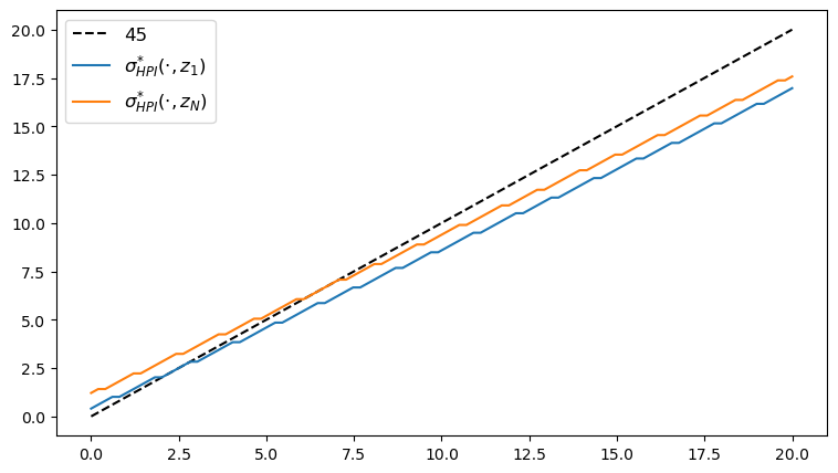
Here’s the plot of the Howard policy, as a function of
fig, ax = plt.subplots(figsize=(9, 5))
ax.plot(y_grid, y_grid, "k--", label="45")
ax.plot(y_grid, y_grid[σ_star_hpi[:, 1]], label="$\\sigma^{*}_{HPI}(\cdot, z_1)$")
ax.plot(y_grid, y_grid[σ_star_hpi[:, -1]], label="$\\sigma^{*}_{HPI}(\cdot, z_N)$")
ax.legend(fontsize=12)
plt.show()
print("Starting VFI.")
%time σ_star_vfi = value_function_iteration(model).block_until_ready()
Show code cell output
Starting VFI.
CPU times: user 573 ms, sys: 11.7 ms, total: 585 ms
Wall time: 648 ms
# Now time it without compile time
start = time()
σ_star_vfi = value_function_iteration(model).block_until_ready()
vfi_without_compile = time() - start
print(σ_star_vfi)
print(f"VFI completed in {vfi_without_compile} seconds.")
[[ 2  2  2 ...  6  6  6]
 [ 3  3  3 ...  7  7  7]
 [ 4  4  4 ...  7  7  7]
 ...
 [82 82 82 ... 86 86 86]
 [83 83 83 ... 86 86 86]
 [84 84 84 ... 87 87 87]]
VFI completed in 0.7083821296691895 seconds.
Here’s the plot of the VFI, as a function of
fig, ax = plt.subplots(figsize=(9, 5))
ax.plot(y_grid, y_grid, "k--", label="45")
ax.plot(y_grid, y_grid[σ_star_vfi[:, 1]], label="$\\sigma^{*}_{VFI}(\cdot, z_1)$")
ax.plot(y_grid, y_grid[σ_star_vfi[:, -1]], label="$\\sigma^{*}_{VFI}(\cdot, z_N)$")
ax.legend(fontsize=12)
plt.show()

print("Starting OPI.")
%time σ_star_opi = optimistic_policy_iteration(model, m=100).block_until_ready()
Show code cell output
Starting OPI.
CPU times: user 500 ms, sys: 9.13 ms, total: 510 ms
Wall time: 552 ms
# Now time it without compile time
start = time()
σ_star_opi = optimistic_policy_iteration(model, m=100).block_until_ready()
opi_without_compile = time() - start
print(σ_star_opi)
print(f"OPI completed in {opi_without_compile} seconds.")
[[ 2  2  2 ...  6  6  6]
 [ 3  3  3 ...  7  7  7]
 [ 4  4  4 ...  7  7  7]
 ...
 [82 82 82 ... 86 86 86]
 [83 83 83 ... 86 86 86]
 [84 84 84 ... 87 87 87]]
OPI completed in 0.20363116264343262 seconds.
Here’s the plot of the optimal policy, as a function of
fig, ax = plt.subplots(figsize=(9, 5))
ax.plot(y_grid, y_grid, "k--", label="45")
ax.plot(y_grid, y_grid[σ_star_opi[:, 1]], label="$\\sigma^{*}_{OPI}(\cdot, z_1)$")
ax.plot(y_grid, y_grid[σ_star_opi[:, -1]], label="$\\sigma^{*}_{OPI}(\cdot, z_N)$")
ax.legend(fontsize=12)
plt.show()

We observe that all the solvers produce the same output from the above three plots.
Let’s plot the time taken by each of the solvers and compare them.
m_vals = range(5, 600, 40)
print("Running Howard policy iteration.")
%time σ_hpi = howard_policy_iteration(model).block_until_ready()
Running Howard policy iteration.
Concluded loop 1 with error 50.
Concluded loop 2 with error 26.
Concluded loop 3 with error 17.
Concluded loop 4 with error 10.
Concluded loop 5 with error 7.
Concluded loop 6 with error 4.
Concluded loop 7 with error 3.
Concluded loop 8 with error 1.
Concluded loop 9 with error 1.
Concluded loop 10 with error 1.
Concluded loop 11 with error 1.
Concluded loop 12 with error 0.
CPU times: user 107 ms, sys: 11.3 ms, total: 118 ms
Wall time: 98.4 ms
# Now time it without compile time
start = time()
σ_hpi = howard_policy_iteration(model).block_until_ready()
hpi_without_compile = time() - start
print(f"HPI completed in {hpi_without_compile} seconds.")
Concluded loop 1 with error 50.
Concluded loop 2 with error 26.
Concluded loop 3 with error 17.
Concluded loop 4 with error 10.
Concluded loop 5 with error 7.
Concluded loop 6 with error 4.
Concluded loop 7 with error 3.
Concluded loop 8 with error 1.
Concluded loop 9 with error 1.
Concluded loop 10 with error 1.
Concluded loop 11 with error 1.
Concluded loop 12 with error 0.
HPI completed in 0.09754800796508789 seconds.
print("Running value function iteration.")
%time σ_vfi = value_function_iteration(model, tol=1e-5).block_until_ready()
Running value function iteration.
CPU times: user 541 ms, sys: 2.75 ms, total: 543 ms
Wall time: 594 ms
# Now time it without compile time
start = time()
σ_vfi = value_function_iteration(model, tol=1e-5).block_until_ready()
vfi_without_compile = time() - start
print(f"VFI completed in {vfi_without_compile} seconds.")
VFI completed in 0.592613935470581 seconds.
opi_times = []
for m in m_vals:
    print(f"Running optimistic policy iteration with m={m}.")
    σ_opi = optimistic_policy_iteration(model, m=m, tol=1e-5).block_until_ready()

    # Now time it without compile time
    start = time()
    σ_opi = optimistic_policy_iteration(model, m=m, tol=1e-5).block_until_ready()
    opi_without_compile = time() - start
    print(f"OPI with m={m} completed in {opi_without_compile} seconds.")
    opi_times.append(opi_without_compile)
Show code cell output
Running optimistic policy iteration with m=5.
OPI with m=5 completed in 0.2438044548034668 seconds.
Running optimistic policy iteration with m=45.
OPI with m=45 completed in 0.18979310989379883 seconds.
Running optimistic policy iteration with m=85.
OPI with m=85 completed in 0.19896388053894043 seconds.
Running optimistic policy iteration with m=125.
OPI with m=125 completed in 0.2048509120941162 seconds.
Running optimistic policy iteration with m=165.
OPI with m=165 completed in 0.22113990783691406 seconds.
Running optimistic policy iteration with m=205.
OPI with m=205 completed in 0.2541649341583252 seconds.
Running optimistic policy iteration with m=245.
OPI with m=245 completed in 0.2799510955810547 seconds.
Running optimistic policy iteration with m=285.
OPI with m=285 completed in 0.29769253730773926 seconds.
Running optimistic policy iteration with m=325.
OPI with m=325 completed in 0.3392040729522705 seconds.
Running optimistic policy iteration with m=365.
OPI with m=365 completed in 0.38036084175109863 seconds.
Running optimistic policy iteration with m=405.
OPI with m=405 completed in 0.4215662479400635 seconds.
Running optimistic policy iteration with m=445.
OPI with m=445 completed in 0.4629220962524414 seconds.
Running optimistic policy iteration with m=485.
OPI with m=485 completed in 0.5038557052612305 seconds.
Running optimistic policy iteration with m=525.
OPI with m=525 completed in 0.5451874732971191 seconds.
Running optimistic policy iteration with m=565.
OPI with m=565 completed in 0.5862724781036377 seconds.
fig, ax = plt.subplots(figsize=(9, 5))
ax.plot(m_vals, jnp.full(len(m_vals), hpi_without_compile),
        lw=2, label="Howard policy iteration")
ax.plot(m_vals, jnp.full(len(m_vals), vfi_without_compile),
        lw=2, label="value function iteration")
ax.plot(m_vals, opi_times, lw=2, label="optimistic policy iteration")
ax.legend(fontsize=12, frameon=False)
ax.set_xlabel("$m$", fontsize=12)
ax.set_ylabel("time(s)", fontsize=12)
plt.show()
